How Do I Compare A Range In Excel?
Di: Samuel
But, Excel’s output doesn’t . Sub Sample() Dim Ar1, Ar2.
Compare two or more worksheets at the same time
Now, select cell A3. Click the ‘Home’ tab.If you have multiple PivotTables, first select any cell in any PivotTable, then on the ribbon go to PivotTable .How to select duplicates in Excel.If two cells equal, return TRUE. Ref (required) – a list of numeric values to rank against.Explanation: this may look a bit overwhelming, but it’s not that difficult. For i = 1, j = 3, Excel VBA compares all values of the .This article uses the following terms to describe the Excel built-in functions: The value to be found in the first column of Table_Array. Here are some of the differences between an Excel Table and Range: Cells in an Excel table need to exist as a contiguous collection of cells.
Filter data in a range or table
Follow the steps to compare two dates in Excel. It will show you which value is greater in two columns. Copy formulas exactly by using Excel’s Find and Replace.
How to Compare Dates in Excel?
In Microsoft Excel, there are many different lookup/reference functions that can help you find a certain value in a range of cells, and MATCH is one of them.If you add new data to your PivotTable data source, any PivotTables that were built on that data source need to be refreshed. First, select cell B3. After that, you will see range B3:C4 is selected as shown below.That is the basic VLOOKUP formula to compare two columns in Excel. Look at the below data to compare dates in Excel. Steps: First, select any cell to place your resultant value. 11-30 will have a score of 2. However, it’s not as simple as that. The first result is if your comparison is True, the second if your comparison is False. Once you filter data in a range of cells or table, you can either reapply a filter to get up-to-date results, or . Depending on your particular task, it can be modified as shown in further examples. Click on cell E5 and insert this formula.One advantage of using this function is that it is case-sensitive.Excel offers a variety of date formatting options.Excel follows general mathematical rules for calculations, which is Parentheses, Exponents, Multiplication and Division, and Addition and Subtraction, or the acronym PEMDAS (Please Excuse My Dear Aunt Sally). Improve this answer. Basically, it identifies a relative position of an item in a range of cells.How to Compare Multiple Columns in Excel.
How to Select a Range of Cells in Excel (9 Methods)
To create a formula that checks if two cells match, compare the cells by using the equals sign (=) in the logical test of IF.Count equals 3, so the first two code lines reduce to For i = 1 to 3 and For j = i + 1 to 3. Dim i As Long, j As Long. Cells in a range, however, don’t necessarily need to be contiguous. Sayyed Abbas Rizvi Sayyed Abbas .
Excel logical operators: equal to, not equal to, greater than, less than
In our example, we will match column List 1 and column List 2.For the first cell in the .You can use the IF function to compare addresses. Then the New Formatting Rule Wizard will appear. So, it is potentially changing the results in that sense.Select a Range of Cells Using Keyboard Shortcut.To use it, you create rules that determine the format of cells based on their values, such as the following monthly temperature data with cell colors tied to cell values.Click on the “View” tab in the Excel ribbon.e integer only Similary time value can be compared with timevalue(s) only. To select duplicate records without column headers, select the first (upper-left) cell, and press Ctrl + Shift + End to extend the selection to the last cell.
How to compare time using Excel VBA
On the Home tab, go to the Editing group, and click Find & Select > . It can be supplied as an array of numbers or a reference to the list of numbers. This is a very small range but still I would recommend using Arrays to store your range values and then use the arrays for comparison. From the drop-down, click on ‘New Rule’. In the Styles group, click on the ‘Conditional Formatting’ option. Returns TRUE if a number in cell A1 is greater than 20, FALSE otherwise.
See this example. I created an export from our CRM system of all companies we have in the CRM system as a single column excel file (column A, .The vlookup with fourth argument of True will find the largets number that does not exceed the number being looked up and requires the leftmost column to be sorted (as shown). Ar1 = Range(A1:A4): Ar2 = Range(B1:B3)
How to compare two columns in Excel using VLOOKUP
Use IF Function to Compare Two Cells. In real life, the columns you need to compare are not always on the same sheet. While your lists are highlighted, in Excel’s ribbon at the top, click the Home tab.In Excel, we can compare dates in two columns which is greater and which is smaller.
IF function
To test if a value exists in a range of cells, you can use a simple formula based on the COUNTIF function and the IF function. Step 1: Select your worksheets and ranges. In the Duplicate Values box, click Duplicate and .Here’s An Complete Example you cant compare an integer with a String an integer value can only be compared with the one with same data type i.Where: Number (required) – the value whose rank you’d like to find.
How to Compare Addresses in Excel (11 Possible Methods)
It may look like IF formulas for dates are the same as IF functions for numeric or text values, since they use the same comparison operators.Other methods are case-insensitive. To scroll both .
Compare Two Lists in Excel for Matches (All Methods and Uses)
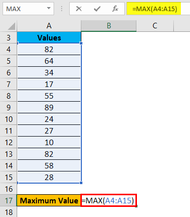
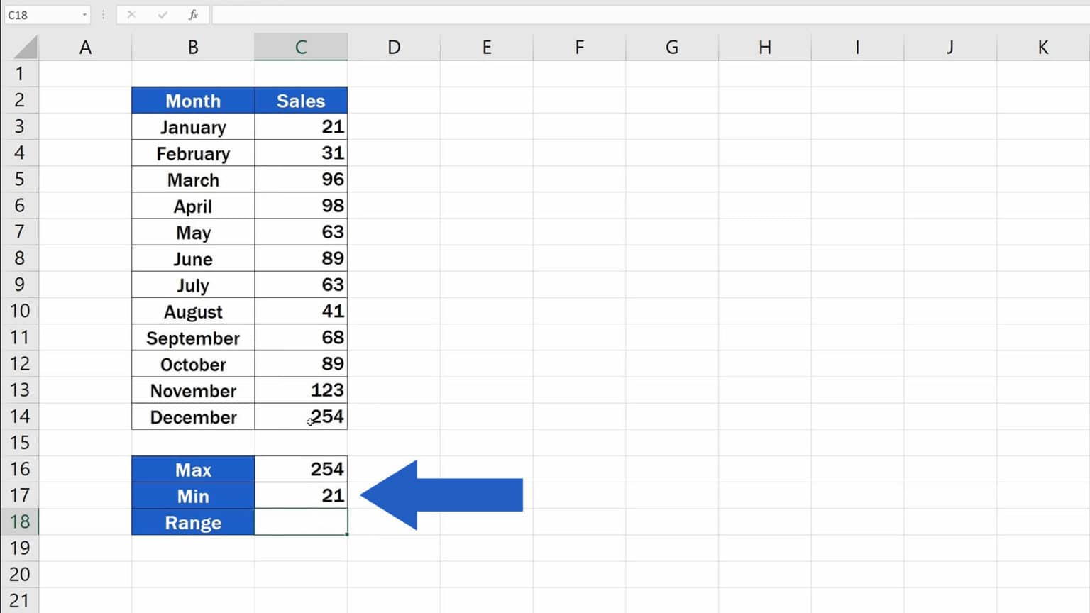
Using the SMALL and LARGE functions to Find the Range of A Series.
How to Perform Regression Analysis using Excel
so since the second number is 11, 0-10 will have a score of 1.
Excel If Time Between Range (4 Quick Ways)
Then you can use =Vlookup (450,D:E,2,True) Comparing whether the date is equal to the other or not is simple; we will have two dates, and we need to check whether that cell date is equal to the other. Excel MATCH function – syntax and basic uses
How to Check If Multiple Cells Are Equal in Excel (4 Methods)
Operators such as , = can be used to compare dates in Excel.Step-01: Select the cell range on which you want to apply the Conditional Formatting (Here, I have selected the column Sales of 2019) Go to Home Tab>> Conditional Formatting Dropdown>> New Rule Option.Drag down the Fill Handle (+) to copy the formula to the rest of the cells. Order (optional) – a number that specifies how to rank values:. Don’t worry if the syntax and argument . =IF(C6=F6,Match,No Match) Formula Explanation. Now you can manually compare the data in each sheet to identify duplicates. Below is the syntax of the XLOOKUP function: =XLOOKUP(lookup_value, lookup_array, return_array, [if_not_found], [match_mode], [search_mode]) If you’ve used VLOOKUP, you’ll notice that the syntax is quite similar, with some awesome additional features of course. Tip: The secret to VLOOKUP is to organize your data so that the value you look up (Fruit) is . With a lower alpha, the p-values must be lower to be significant. This allows me to quickly and easily loop over a Range of cells easily: Dim r As Long. assume these start in D1 and E1. The column number in Table_Array the matching value should be returned for. The simplest If one cell equals another then true Excel formula is this: cell A = cell B. The range of cells that contains possible lookup values. It interprets them as regular text values. For example: =A1>20. Dim Found As Boolean. Use ⬆ or ⬅ to select cells above or left to the first cells respectively. The IF function is one of the most popular functions in Excel, and it allows you to make logical comparisons between a value and what you expect.I’m not really sure why Excel asks for alpha. Then, type the following formula in the selected cell or in the Formula Bar. For i = 1, j = 2, Excel VBA compares all values of the first area with all values of the second area. If the needed worksheet is not in the list, click the Open Workbook button above the list and open the Excel file you need. Compare two columns in different Excel sheets using VLOOKUP. As the result, you’ll get TRUE if two cells are the same, FALSE otherwise:
vba
Select Use a formula to determine which cells to format option. Type in the formula: =LARGE (B2:B7,1) – SMALL (B2:B7,1) Press the Return key. After that, press ENTER to get the output.
How to Compare Two Columns in Excel (for matches
There are four different types of calculation operators: arithmetic, comparison, .

Like AND function this function is also used . Under Input Y Range, select the range for your dependent variable. value_if_true: Describe what should occur if the test result is TRUE.
How to Compare Two Excel Sheets for Duplicates: 5 Quick Ways
? Steps: Select cell D5 and write down =B5>C5. Alternatively, highlight the desired range, select the Formulas tab on the ribbon, then select Define Name. With Sheet1 ‚ <-- You should always qualify . For example, =IF (C2=”Yes”,1,2) says IF (C2 = Yes .Step-by-Step Instructions for Filling In Excel’s Regression Box. As the formula is copied down it returns Yes if the value in column E . In the list of open books, select the sheets you are going to compare.Arrange multiple Excel windows side by side. The dependent variable is a variable that you want to explain or predict . So an IF statement can have two results.Using IF Function with Dates in Excel. In this dialog box, under Compare Side by Side with, click the workbook that contains the worksheet that you want to compare with your active worksheet, and then click OK. That can change which group comparisons end up being statistically significant. How do you put 3 conditions in the IF function in Excel? value_if_false: Define what should occur if the test result is FALSE. In the ‘New Formatting Rule’ dialog box, click on the ‘Use a .The IF function in Microsoft Excel has three parts (arguments): logical_test: compares something, such as a cell’s value.
Using IF Function with Dates in Excel (Easy Examples)
Using parentheses allows you to change that calculation order. I selected cell H5.Below is the formula that will do this: =IF(C2<=B2,In Time,Delayed) The above formula compares the two dates using the less than or equal to operator, and if the submission date is before the due date, it shows ‘In Time’, else it shows delayed. Use Excel EXACT Function to Check If Multiple Cells Are Equal. Then select cell E5 and write down B5 Otherwise, the formula must be entered as a legacy array formula by first selecting the . Press Enter to get the result. Now in cell C2, apply the formula as =A2=B2. Likewise, equal to a sign, you can find matches/mismatches using this function.To use the method, first, select the lists you want to compare in your spreadsheet.XLOOKUP Function Syntax. To compare dates in Excel, we will use logical operators to check whether the two dates match or not. Highlight the desired range of cells and type a name in the Name Box above column A in the worksheet. The EXACT function is used to check if comparing cell values are the same or not. To view all open Excel files at a time, . Select the cells with the formulas that you want to copy. For example, to compare cells in columns A and B in each row, you enter this formula in C2, and then copy it down the column: =A2=B2. On the Home tab, in the Styles section, click Conditional Formatting > Highlight Cells Rules > Duplicate Values.Here are the steps to do this: Select the entire dataset. The Compare Side by Side dialog box will appear, and you select the files to be displayed together with the active workbook. By default, the tool compares the used ranges of the sheets.This will give True or False at the output cell. Find Matches in All Cells Within the Same Row. Follow answered Jan 25, 2016 at 5:06. We will have a new column named Matching Status.Use the following procedure, which uses the logical Equal (=) operator to determine that. A range that contains only one row or column. Using Logical Operator. Unfortunately, unlike other Excel functions, the IF function cannot recognize dates. “Vertical” or “Horizontal”.Note: Dynamic array formulas – If you have a current version of Microsoft 365, and are on the Insiders Fast release channel, then you can input the formula in the top-left-cell of the output range, then press Enter to confirm the formula as a dynamic array formula. To find the range of values in the given dataset, we can use the SMALL and LARGE functions as follows: Select the cell where you want to display the range (B8 in our example). To select duplicates, including column headers, filter them, click on any filtered cell to select it, and then press Ctrl + A. In each workbook window, click the sheet that you want to compare. Choose an arrangement option e. =A1>= (B1/2) Returns TRUE if a number in cell A1 is greater than or equal to the quotient of the division of B1 by 2, FALSE otherwise. Click on “Arrange All” in the “Window” group. Common date functions in Excel include TODAY (), MONTH (), YEAR (), and DATE (). If same, it will return TRUE, otherwise FALSE. =XLOOKUP (lookup_value, lookup_array, return_array, [if_not_found], [match_mode], [search_mode]) *If omitted, XLOOKUP returns blank cells . You can press the arrows more times to extend the selection. To refresh just one PivotTable, you can right-click anywhere in the PivotTable range, and then select Refresh. In the example shown, the formula in F5, copied down, is: = IF ( COUNTIF ( data,E5) > 0,Yes,No) where data is the named range B5:B16. You can apply conditional formatting to a range of cells (either a selection or a named range), an Excel table, and in Excel for Windows, even a PivotTable report. Press ENTER and drag down Fill Handle. To view more than 2 Excel files at a time, open all the workbooks you want to compare, and click the View Side by Side button. In Loops, I always prefer to use the Cells class, using the R1C1 reference method, like this: Cells(rr, col). If no match exists, then XLOOKUP can return the closest (approximate) match. If you have more than two workbooks open, Excel displays the Compare Side by Side dialog box. For example: =IF(B2=C2, Same score, ) To check if the two cells contain same text including the letter case, make your IF formula case-sensitive with the help of the EXACT function.Just select the data, along with the labels, and use the Create from Selection command on the Formulas tab of the ribbon: You can also use the keyboard shortcut control + shift + F3. Then press SHIFT+ + ⬇.In its simplest form, the VLOOKUP function says: =VLOOKUP (What you want to look up, where you want to look for it, the column number in the range containing the value to return, return an Approximate or Exact match – indicated as 1/TRUE, or 0/FALSE). This will display both sheets either side by side or one above the other.Most often, Excel comparison operators are used with numbers, date and time values.Not only do they look different, they are also quite different in the amount of functionality they offer. Comparing by company name only.Use AutoFilter or built-in comparison operators like greater than and “top 10” in Excel to show the data you want and hide the rest.The XLOOKUP function searches a range or an array, and then returns the item corresponding to the first match it finds. To copy a range of Excel formulas without changing their cell references, you can use the Excel Find and Replace feature in the following way. What you need to do is compare the p-values to your alpha. However, the MATCH function can do much more than its pure essence. =IF(AND(B5=C5, B5=D5), Complete match, ) If all three columns in the same row have the same data, the result will be a Complete match. The formula to compare dates in Excel is =A1>B1, where A1 and B1 are the cells containing the dates you want to compare. To manage range names, go to the Formulas tab, select Name Manager, choose a name, then select Delete or Edit. If 0 or omitted, the values are ranked in descending order, i.Click the Agree button to continue.I am tasked with comparing the Attendee list/spreadsheet with our company CRM database to see if they are already in the system.
How to Compare Dates in Two Columns in Excel (8 Methods)
Value exists in a range

Excel if match formula: check if two or more cells are equal